Hot Ones, a renowned American YouTube talk show, was conceived by Chris Schonberger and is expertly hosted by Sean Evans. The show is a production of First We Feast and Complex Media. At its core, Hot Ones orchestrates engaging interviews with celebrities, set against the backdrop of a progressively spicier array of chicken wings. This intriguing premise has birthed various offshoots, including Hot Ones: The Game Show on TruTV, a cable television network, as well as Truth or Dab, an inventive truth or dare-style contest featured on the First We Feast YouTube channel.
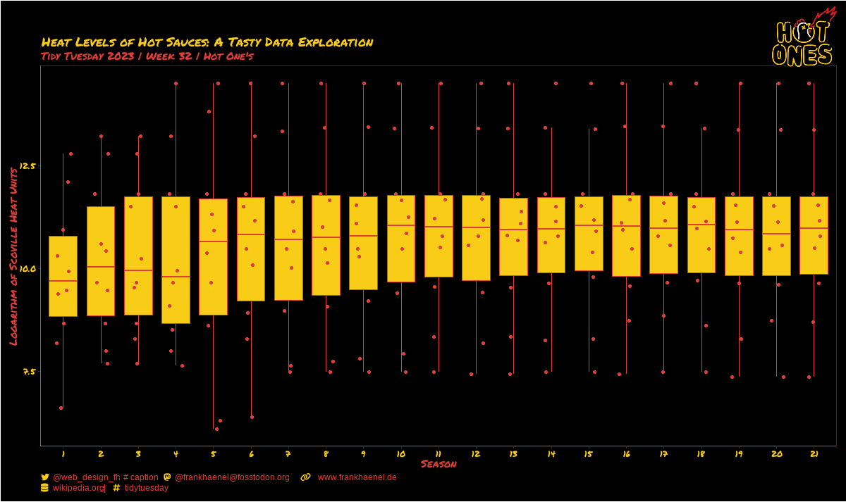
Inspired by the captivating world of Hot Ones, I embarked on an exploration into the Heat Levels of Hot Sauces using illuminating boxplots.
Loading packages, data, fonts and difining colors
library(tidyverse)
library(showtext)
library(glue)
library(ggtext)
library(magick)
library(grid)
library(tidytuesdayR)

tuesdata <- tidytuesdayR::tt_load(2023, week = 32)
##
## 	Downloading file 1 of 3: `episodes.csv`
## 	Downloading file 2 of 3: `sauces.csv`
## 	Downloading file 3 of 3: `seasons.csv`
sauces <- tuesdata$sauces # fonts and colors font_add('fa-reg', 'c:/Users/info/OneDrive/Dokumente/fonts/Font Awesome 6 Free-Regular-400.otf') font_add('fa-brands', 'c:/Users/info/OneDrive/Dokumente/fonts/Font Awesome 6 Brands-Regular-400.otf') font_add('fa-solid', 'c:/Users/info/OneDrive/Dokumente/fonts/Font Awesome 6 Free-Solid-900.otf') font_add_google("Permanent Marker", "pm") showtext_auto() col <- c("#F9CC17","#DD3E37","black") col1 <- col[1] col2 <- col[2] bg <- col[3] # text creation twitter <- glue("<span style='color:{col1};font-family:fa-brands;'></span>") mastodon <- glue("<span style='color:{col1};font-family:fa-brands;'></span>") link <- glue("<span style='color:{col1};font-family:fa-solid;'></span>") data <- glue("<span style='color:{col1};font-family:fa-solid;'></span>") hash <- glue("<span style='color:{col1};font-family:fa-solid;'>#</span>") space <- glue("<span style='color:{bg}'>-</span>") space2 <- glue("<span style='color:{bg}'>--</span>") # can't believe I'm doing this t <- "Heat Levels of Hot Sauces: A Tasty Data Exploration" # title s <- "Tidy Tuesday 2023 | Week 32 | Hot One's" # subtitle cap <- glue("{twitter}{space2}@web_design_fh{space2} # caption {space2}{mastodon}{space2}@frankhaenel @fosstodon.org{space2} {space2}{link}{space}{space2}www.frankhaenel.de<br> {data}{space2}wikipedia.org{space2}| {space2}{hash}{space2}tidytuesday")
Plot
        sauces %>% ggplot(aes(x=as.factor(season), y=log(scoville))) +
                geom_boxplot(color=col2,fill=col1,outlier.color = bg) +
                geom_jitter(shape=16, position=position_jitter(0.2), color=col2) +
        theme_bw() +
        theme(
                axis.line = element_line(color = col2),
                axis.line.x.top = element_line(color = bg),
                axis.line.y.right = element_line(color = bg),
                axis.title = element_text(color = col2,family = "pm"),
                axis.text = element_text(color = col1,family = "pm"),
                panel.grid.major = element_blank(), panel.grid.minor = element_blank(),
                panel.background = element_rect(fill=bg),
                plot.background = element_rect(fill=bg),
                plot.title = element_text(color = col1,family = "pm"),
                plot.subtitle = element_text(color = col2,family = "pm"),
                plot.caption = element_markdown(color = col2,hjust = 0, lineheight = 1.3),
                plot.margin = margin(t = 40,  # Top margin
                             r = 10,  # Right margin
                             b = 10,  # Bottom margin
                             l = 10)) +
        labs(
        title = t,
        subtitle = s,
        caption = cap,
        x = "Season",
        y = "Logarithm of Scoville Heat Units"
        )
        logo <- image_read("C:/Users/info/OneDrive/Dokumente/632-6321331_hot-ones-logo-transparent-hd-png-download.png")
        grid::grid.raster(logo, x = 0.99, y = 0.99, just = c('right', 'top'), width = unit(1, 'inches'))

